Problem Overview
The question that this workflow addresses is how to create a one-second Seamless Coastal Digital Elevation Model (SCDEM) from one-meter resolution raster images derived from LiDAR surveys? While there are already some automated scripts and manual processes using ArcMap, the main challenge is how to completely automate the process.
Solution Overview

Our workflow was tested on a key part of the process used by Geoscience Australia (GA) used to construct the national Australian DEM (digital elevation model), itself a component of the national Australian Foundational Spatial Data Framework (FSDF).
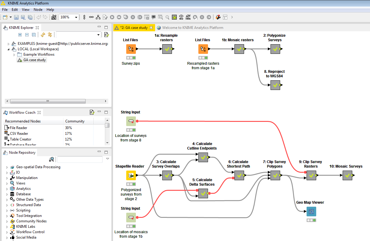
As you can see above, our solution includes 10 steps as follows:
- Resample and Mosaic surveys: Surveys are first ranked according to their age. Within each survey, there is a set of raster tiles that make up that survey. Each of these tiles are resampled to a resolution of 25x25m, with each tile named sequentially and placed in its own rank folder to avoid duplicate filenames. Next, for each survey, every resampled tile within that survey is taken and joined into a single image mosaic named after that survey’s rank.
- Polygonise surveys: Polygonisation is a two step process that involves first creating a mask raster image for each mosaicked survey to indicate which pixels are within the survey, and then creating shapefiles for each of these rasters to represent their boundaries as polygons. These shapefiles are then merged, to create a single shapefile containing all surveys.
- Calculate survey overlaps: This stage determines where survey polygons overlap. It does so by finding pairs of survey polygons where the first is more recent (i.e., has a higher rank) than the second, with geometries that overlap. Any linestrings present in the overlapping geometries are removed, the overlapping polygons are split into individual polygons (in some cases, two surveys may overlap multiple times).
- Calculate cutline endpoints: In order to calculate the cutlines between surveys, the endpoints of these lines must first be determined. This stage automates finding these endpoints by implementing a few simple rules.
- Calculate delta surfaces: Calculating the delta surfaces is a two step process that first clips the overlapping rasters to the bounding box of the overlap polygon before combining these two rasters to make the delta surface.
- Calculate shortest path: This stage uses the R package gdistance , to calculate the least cost shortest path through each delta surface between the corresponding cutline endpoints using Dijkstra’s algorithm.
- Clip survey polygons: This stage takes the overlap polygons and cutlines from stages 3 and 6 and applies them to the survey polygons to define the clipped extent of each survey. Given that each cutline will split the overlapping areas between surveys, if the outermost parts are found for each survey, then they can be removed from that survey to create clipped polygons.
- Reproject to WGS84: This stage reprojects each survey to WGS84 with a 1-degree cell size as this is the coordinate reference system and resolution used by the national DEM.
- Clip survey rasters: This stage clips the projected raster images from stage 8 to the extent of the polygons from stage 7, ensuring that no survey overlaps.
- Mosaic surveys: The final stage joins each clipped survey raster into a single image mosaic.
MAC/Linux Users
Please note that on mac/linux platforms you might experience some issues with KNIME. The reason is that KNIME cannot find the GDAL path in the PATH variable. If this issue happens, please open an terminal and access the KNIME application by executing the following command:
open /Applications/KNIME\ 3.3.2.app/
This way the PATH variable is shared with the KNIME application and you can run the workflows successfully.
Download Resources
The GA workflow can be downloaded from here. The input data includes the 13 following surveys stored in individual zip files. Each survey containing a collection of 1x1km tiles in ESRI ARC/INFO Binary Grid format.
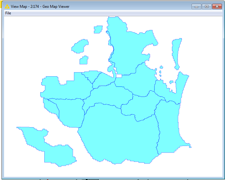
Output
The following view can be obtained by GeoMapViewer Node.
Our workflow was tested on a key part of the process used by GA used to construct the national Australian DEM (digital elevation model), itself a component of the national Australian Foundational Spatial Data Framework (FSDF).